Sampling, Antialiasing, and Monte Carlo

A single sample at the center of each pixel may produce a recognizable first image, but it cannot represent the spatial variation present at silhouette edges, narrow specular highlights, or high-frequency textures; the resulting errors appear as stair-stepping, aliasing, and temporal sparkle under motion.

The initial remedy is not a post-process blur, but a correct sampling strategy and linear-space average over the pixel footprint.

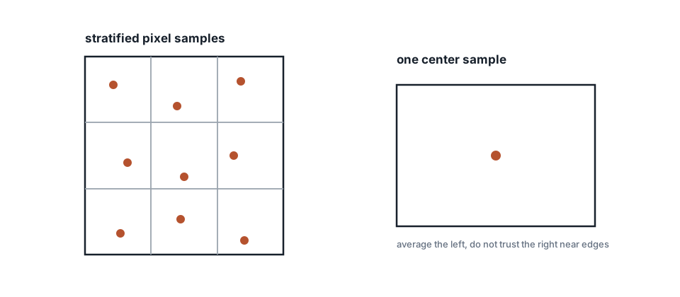
Several stratified samples inside a pixel beat one center sample near edges.

Pixel antialiasing

color = 0
for k = 1..N:
    (s, t) = stratified or random in [0, 1)²
    ray = camera.generate(i, j, s, t)
    color += trace(ray)
color /= N

Stratified sampling partitions the pixel into cells and places one sample within each cell, thereby reducing the clumping characteristic of purely uniform random samples. Blue-noise patterns can provide improved visual behavior when available, but stratification is sufficient for establishing the estimator and its variance properties.

Monte Carlo estimation

To approximate an integral, sample the domain and average carefully:

$$ \int f(x),dx \approx \frac{1}{N}\sum_{i=1}^{N}\frac{f(x_i)}{p(x_i)} $$

Here $p$ denotes the probability density that generated $x_i$. Omitting this factor makes image brightness depend on the sampling strategy rather than the underlying integral, a bias that can remain deceptively plausible when only relative contrast is inspected.

Light sampling and BSDF sampling

Direct lighting can sample lights. Indirect lighting often samples the BSDF. Ideal mirrors must be sampled by their reflection direction. Random hemisphere directions will almost never hit a Dirac lobe.

A practical teaching order:

1. stratified pixel samples
2. one analytic light with shadow rays
3. cosine-weighted hemisphere samples for diffuse indirect light
4. multiple importance sampling only after the above are correct

Cosine-weighted hemisphere

Uniform hemisphere sampling wastes effort near the horizon, where cosθ kills the contribution. For Lambertian surfaces, cosine-weighted sampling matches the integrand better:

$$ \begin{aligned} r_1,r_2 &\sim U(0,1) \ \phi &= 2\pi r_1 \ r &= \sqrt{r_2} \ x &= r\cos\phi,\quad y = r\sin\phi,\quad z = \sqrt{\max(0,1-r_2)} \ p &= \frac{z}{\pi} \end{aligned} $$

Transform (x,y,z) into world space with a basis around n. For Lambert, f cosθ / pdf simplifies cleanly. If the simplified result disagrees with brute-force evaluation, the sampler is wrong.

Noise versus bias

Too few samples produce noise. A missing PDF term or an energy clamp produces bias. Denoisers hide noise. They cannot invent the correct mean of a wrong estimator. Prefer a noisy correct image while debugging.

Temporal behavior

Still frames conceal crawling edges. Camera motion reveals them. Per-frame white noise shimmers. Stable sequences are a later topic. Honesty of the still estimator comes first.

Common errors

• Randomizing only one pixel axis
• Averaging sRGB values instead of linear values
• Hemisphere samples without the matching PDF
• Using 1/N while forgetting 1/pdf
• Enabling a denoiser before high-sample raw accumulation is trustworthy

If increasing sample count lowers noise without shifting average brightness, the estimator is probably sane.

Expected value intuition

If each sample is an unbiased estimate of pixel radiance, the average of N samples is also unbiased and its variance falls roughly like 1/N for independent samples. That is why four times the samples halves the RMS noise only in the independent case, and why structured samplers can look better sooner. You are estimating an integral. You are not “drawing harder.”

Domain checklist

State the domain before coding a sampler:

• pixel area
• lens disk
• light area
• hemisphere around n
• time interval

Each domain has a measure and a PDF. If you cannot write the PDF, you are not finished designing the sampler.