Path Tracing in Practice

Path tracing is the point at which the preceding subjects become one transport algorithm. The camera supplies initial rays, the acceleration structure determines visibility, materials determine how paths continue, and the film accumulates weighted radiance estimates. The purpose of the integrator is not to simulate every physical detail explicitly, but to construct an unbiased or acceptably controlled estimator of the reflection equation.

All accumulation must remain linear. Each sample estimates radiance for a pixel footprint, the film adds these estimates, and the display transform is applied only after the accumulated value has been divided by the number of samples. This distinction is fundamental: tone mapping inside the sampling loop changes the estimator rather than merely changing the presentation.

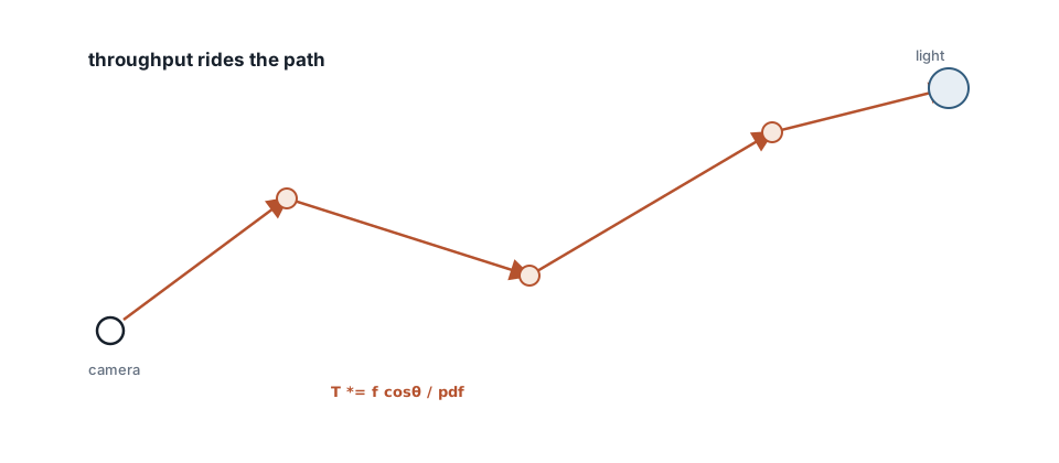
Throughput is the multiplicative weight that carries a path contribution from the camera to its current vertex.

Integrator structure

A conventional iterative path tracer has the following structure:

for each sample:
    ray = camera ray
    throughput = 1
    color = 0
    for bounce = 0..max_depth:
        hit = scene.intersect(ray)
        if no hit:
            color += throughput * environment(ray)
            break

        color += throughput * emission(hit)

        wi, pdf, f = sample_material(hit, -ray.dir)
        if pdf == 0 or f == 0: break
        throughput *= f * cos_theta / pdf

        if bounce >= 3:
            q = clamp(max_component(throughput), 0.05, 0.95)
            if random() > q: break
            throughput /= q

        ray = Ray(offset(hit), wi)

    accumulate(color)

The throughput term contains the product of BRDF values, cosine factors, and reciprocal probability densities encountered along the path. It answers a simple question with significant consequences: if a light source is found after several scattering events, how much of that emitted radiance can still contribute to the original camera sample? A missing cosine, PDF, or visibility term does not merely alter the appearance of the image; it changes the estimator.

Direct-light sampling and Russian roulette

A path that reaches a light only by chance is mathematically valid but often impractically noisy, particularly for small emitters. Next-event estimation addresses this problem by sampling a light explicitly at each non-specular surface, testing the corresponding shadow ray, and adding its weighted contribution. Specular paths must still be sampled through the BSDF because a light sampler cannot, by itself, discover the measure-zero mirror direction required by an ideal reflection or refraction.

Russian roulette provides a probabilistic termination rule for long paths. If a path survives with probability $q$, its remaining throughput must be divided by that same probability:

$$ T\leftarrow\frac{T}{q}. $$

This compensation preserves the expected value of the estimate. Without it, the image systematically darkens as soon as roulette begins. Roulette is usually deferred until several bounces have been evaluated, because early path vertices often carry substantial energy and terminating them merely increases variance.

Film accumulation and diagnostic boundaries

The film owns sample accumulation and output conversion:

buffer[pixel] += sample
display = tone_map(buffer[pixel] / sample_count)

Rare, high-contribution samples are usually called fireflies. Their presence should initiate an investigation of sampling distributions, emitter geometry, and BSDF weights before clamping is introduced, since clamping trades variance for bias. The renderer benefits from clear ownership boundaries: Camera generates rays, Scene or BVH answers intersection queries, Material samples and evaluates scattering, Integrator owns transport estimation, and Film owns accumulation and presentation. These boundaries make a wrong image diagnosable rather than merely disappointing.

Acceptance criteria

A useful validation sequence begins with normal-colored primary hits under the same camera used by the final integrator, then proceeds through a diffuse enclosure whose brightness does not change with sample count, a mirror that reflects emitters and geometry sharply, and a dielectric that handles reflection, refraction, and total internal reflection without black edge artifacts. Increasing the sample count from 16 to 256 should reduce variance while leaving the expected brightness stable. If the mean drifts as samples accumulate, the problem is ordinarily a missing PDF, incorrect averaging, premature display conversion, or an unaccounted selection probability.

A production renderer eventually adds multiple importance sampling, adaptive strategies, denoising, and specialized GPU execution paths. Those techniques are valuable only after the reference estimator is trustworthy. Maintaining a slower CPU reference integrator remains one of the most effective ways to adjudicate disagreements with a faster SIMD or GPU path, because a plausible low-sample image is not evidence that the underlying estimator is correct.